Index
Lecture2
Note for Coursera Machine Learning made by Andrew Ng.
Linear regression with one variable
Model representation
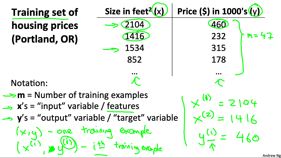
We use House price pridiction as our example
We use following notations
- m = Number of training examples
- x’s = “input” variable / features
- y’s = “output” variable / “target” variable
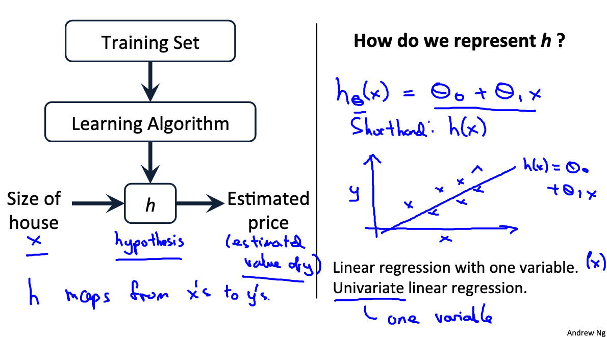
The following figure shows how we get the estimated price and how do we represent h.
Link to coursera section
https://www.coursera.org/learn/machine-learning/supplement/cRa2m/model-representation
Cost function intuition I
Cost Function
We can measure the accuracy of our hypothesis function by using a cost function. This takes an average difference (actually a fancier version of an average) of all the results of the hypothesis with inputs from x’s and the actual output y’s.
To break it apart, it is the difference between the predicted value and the actual value.
This function is otherwise called the “Squared error function”, or “Mean squared error”. The mean is halved
Example
Suppose we have a training set & use linear model then we have
The idea is to choose
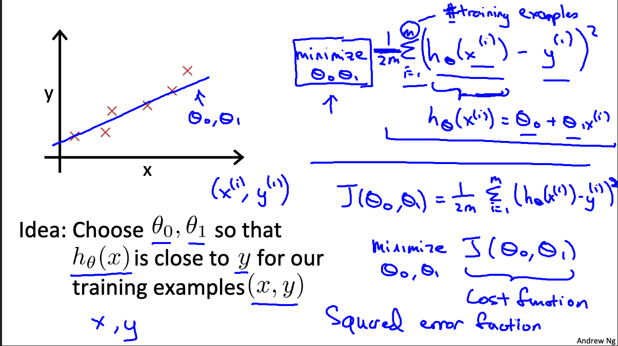
- The goal here is to find
that produce a cost function that has minimum value.
Link to coursera section
https://www.coursera.org/learn/machine-learning/supplement/nhzyF/cost-function
Cost function intuition II
- Hypothesis:
- Parameters:
- Cost Function:
- Goal: minimize
Contour figures

A contour plot is a graph that contains many contour lines. A contour line of a two variable function has a constant value at all points of the same line. An example of such a graph is the one to the right below.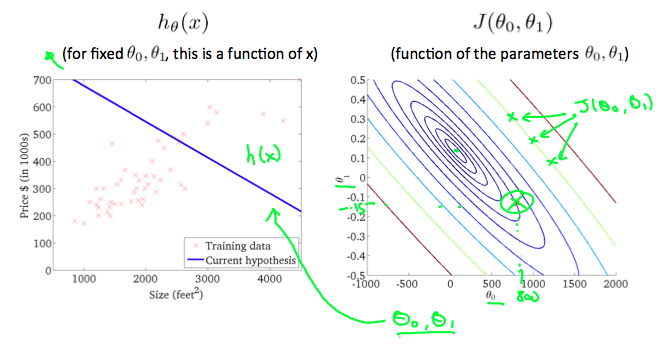
The following figure shows the minimum of the cost function.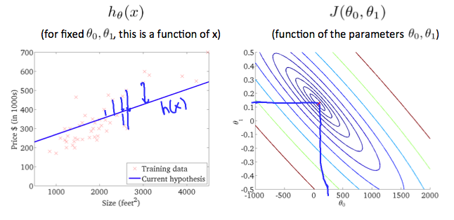
Link to coursera section
https://www.coursera.org/learn/machine-learning/supplement/9SEeJ/cost-function-intuition-ii
link about contour representation :
Gradient descent
Outline:
- Start with some
- Keep changing
to reduce until we hopefully end up at a minimum.
However, givien a different initial values might end up with different minimum(local minimum). This algorithm does not guarantee to be end up at global minimum.
See the following figures.
This figure end up with a local minimum which is also the global minimum in this case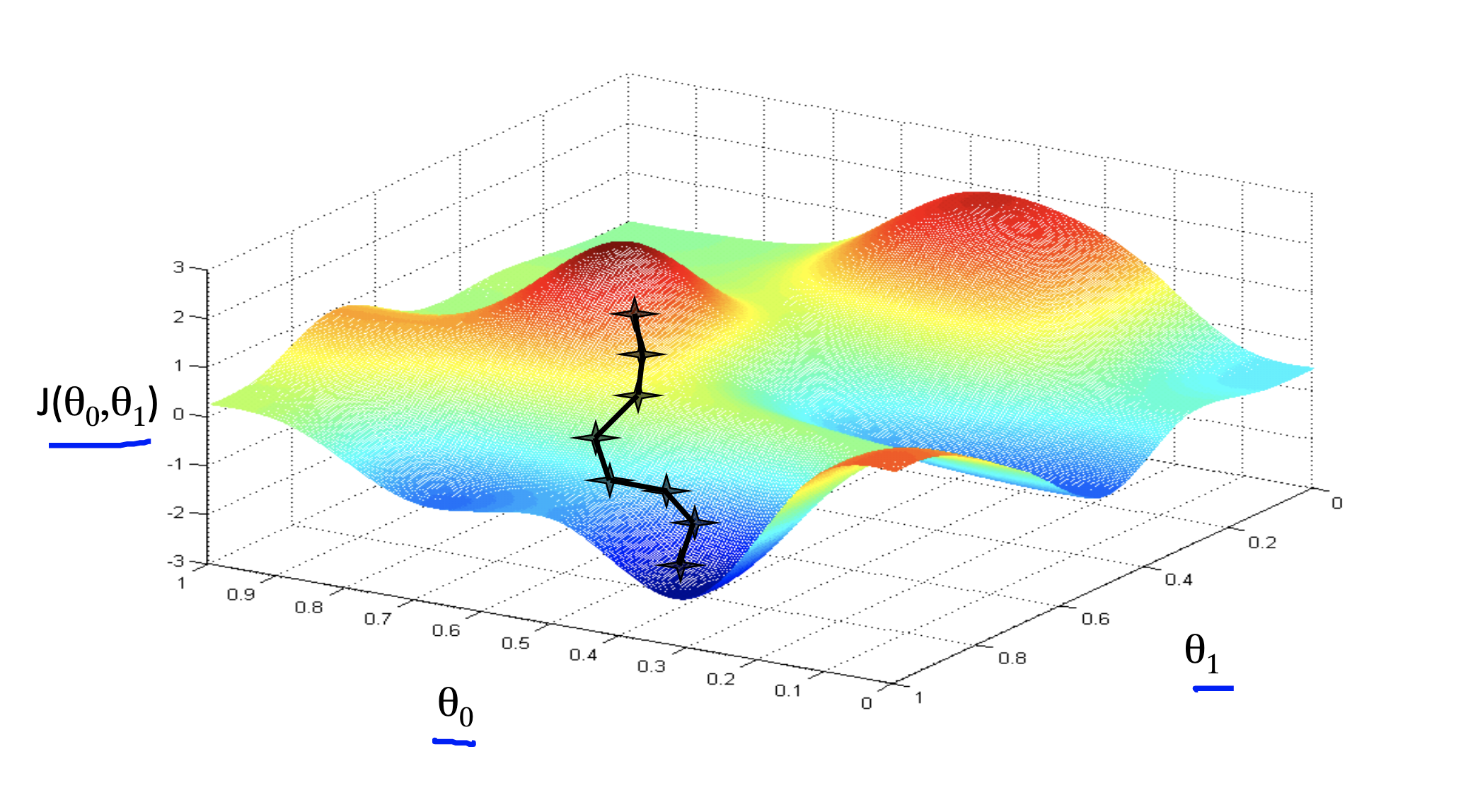
If we choose another inital point, it might end up with a local minimum which is not the global minimum.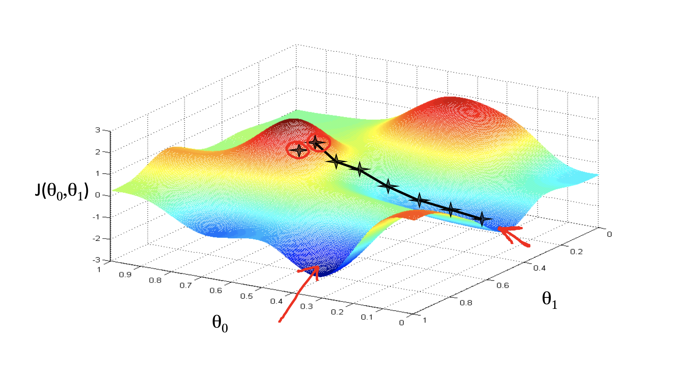
Link to coursera section
https://www.coursera.org/learn/machine-learning/supplement/2GnUg/gradient-descent
Gradient descent intuition
Gradient descent algorithm
repeat until convergence {
}
is the learning rate
Gradient descent with different
see belowing figure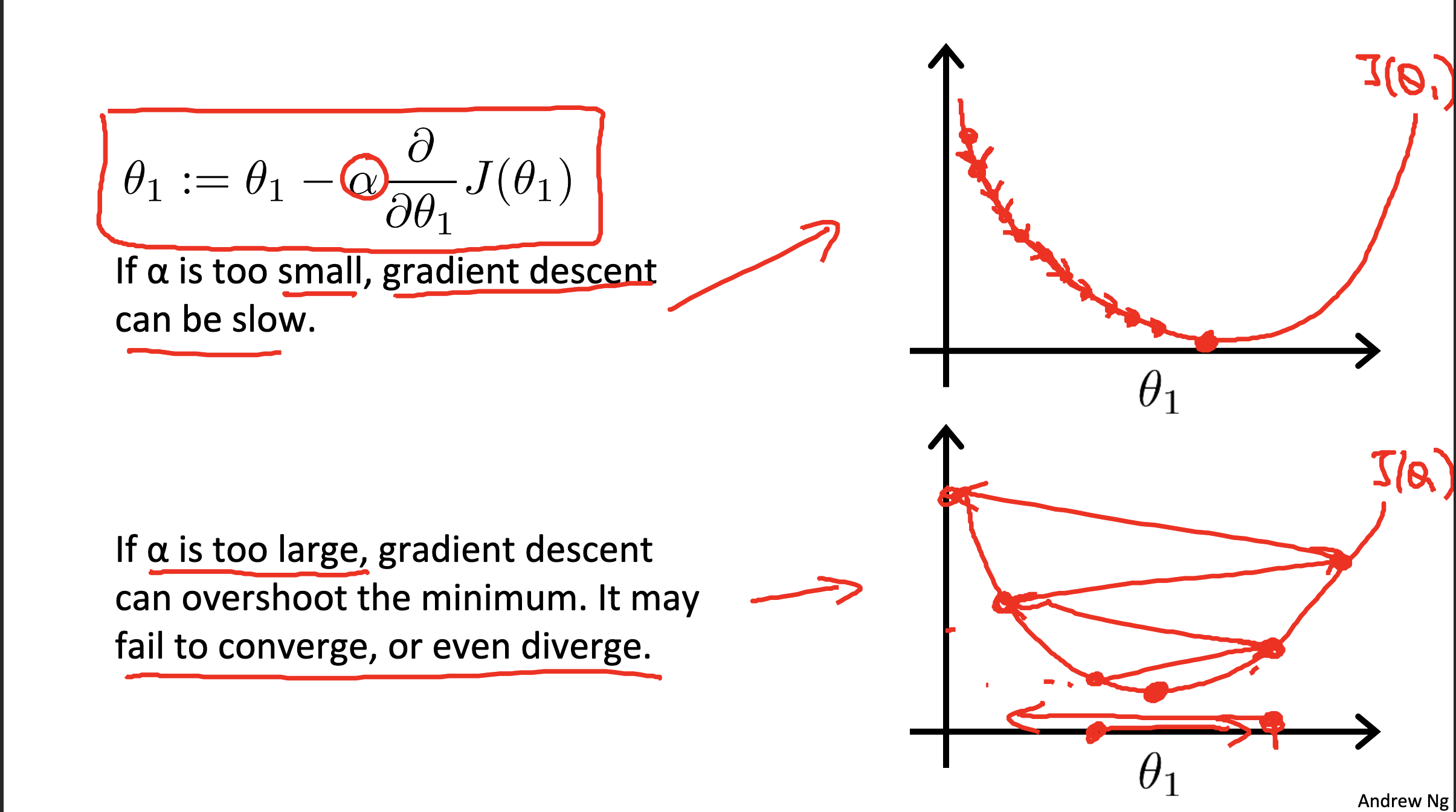
We don’t need to change the value of
see belowing figure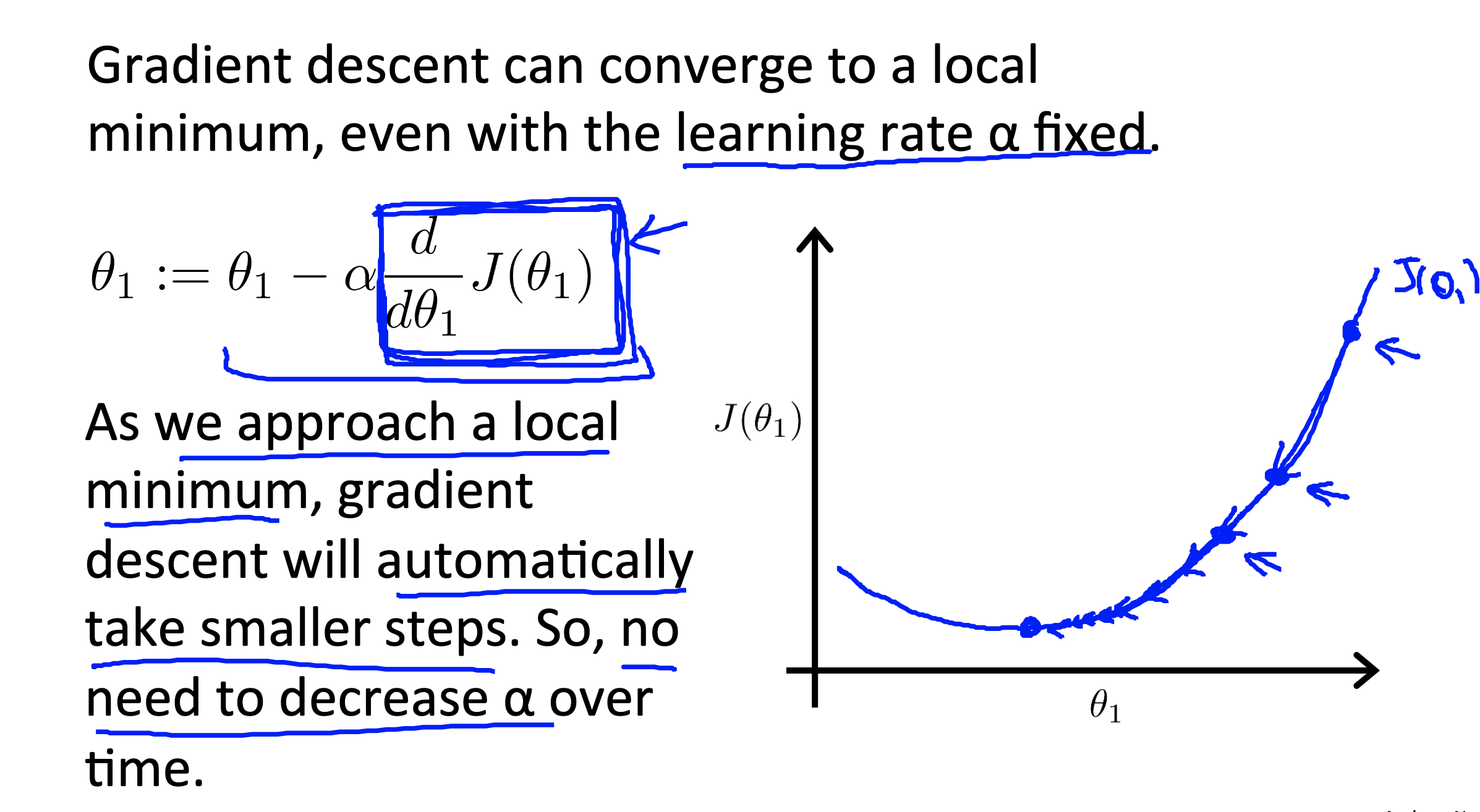
Link to coursera section
https://www.coursera.org/learn/machine-learning/supplement/QKEdR/gradient-descent-intuition
Gradient descent for linear regression
Check coursera for main reading content
Link to coursera section
Some proof
Linear Algebra Review
Link to coursera section
- Matrices and Vectors - https://www.coursera.org/learn/machine-learning/supplement/Q6mSN/matrices-and-vectors
- Addition and Scalar Multiplication - https://www.coursera.org/learn/machine-learning/supplement/FenyC/addition-and-scalar-multiplication
- Matrix-Vector Multiplication - https://www.coursera.org/learn/machine-learning/supplement/cgVgM/matrix-vector-multiplication
- Matrix-Matrix Multiplication - https://www.coursera.org/learn/machine-learning/supplement/l0myT/matrix-matrix-multiplication
- Matrix Multiplication Properties - https://www.coursera.org/learn/machine-learning/supplement/Xl0xT/matrix-multiplication-properties
- Inverse and Transpose - https://www.coursera.org/learn/machine-learning/supplement/EcNto/inverse-and-transpose

Sukoshi
贵在坚持
23
4
23